library(tidyverse)
library(posterior)
library(cmdstanr)
library(ggplot2)
Consider the problem of finding the best player or deck in a game based on match outcomes. A naive approach is to rank by their win rates, without taking anything else (other than possibly computing marginal confidence intervals) into account. This can be misleading, particularly when some candidates have few matches: observed differences may simply reflect chance rather than true differences in quality, which will not be properly accounted for in a marginal confidence interval.
The proposed solution in this blog is to consider all candidates simultaneously using a hierarchical Bayesian multinomial model, which allows for partial pooling of information across candidates. This model will shrink extreme estimates towards the overall mean, with the shrinkage amount depending on the amount of data available for each candidate.
Note
Note, that these types of questions are typically framed as is “A better than B?”, ignoring the process that led to asking this question (i.e. the full set of candidates and their outcomes). A and B are chosen because they are the ones with observed best performance, which is likely an overestimate of their true performance. This is known as winner’s curse. For instance, consider the case where we have \(K=50\) candidates in total. The first \(49\) candidates each have a true win rate of \(0.5\), with \(n_k = 20\) observations for \(k = 1, \dots, 49\). The last candidate has a true winrate of \(0.7\) with \(n_{50}=100\) observations. We simulate observed wins and losses for each candidate:
set.seed(1405)
K <- 50
n <- c(rep(20, K - 1), 100)
true_winrates <- c(rep(0.5, K - 1), 0.7)
observed_wins <- rbinom(K, n, true_winrates)
observed_losses <- n - observed_wins
observed_winrates <- observed_wins / n
data.frame(
  candidate = 1:K,
  True_Winrate = true_winrates,
  Observed_Winrate = observed_winrates
) |>
  arrange(desc(Observed_Winrate)) |>
  head(10)
candidate True_Winrate Observed_Winrate
1 31 0.5 0.80
2 23 0.5 0.75
3 46 0.5 0.70
4 27 0.5 0.65
5 29 0.5 0.65
6 50 0.7 0.62
7 6 0.5 0.60
8 7 0.5 0.60
9 20 0.5 0.60
10 32 0.5 0.60We see, that the candidate with true winrate \(0.7\) is not even in top \(5\) of the observed winrates. Thus, asking a question like “Is candidate A better than candidate B?” without considering the full data generating process (DGP) can lead to misleading conclusions.
Setup
Suppose we observe \(K\) candidates (e.g., players, decks, etc.). Each observation falls into one of \(C\) categories, such as “win”, “loss”, or “tie” in a game context. For each candidate \(k \in \{1, \ldots, K\}\), let \[y_{k} = (y_{k1}, y_{k2}, \ldots, y_{kC})\] denote the observed counts in each category, with total \[n_k=\sum_{c=1}^{C} y_{kc}.\] We model the counts using a multinomial distribution: \[y_k \sim \text{Multinomial}(n_k, \pi_k),\] where \[\pi_k = (\pi_{k1}, \pi_{k2}, \ldots, \pi_{kC}), \quad \sum_{c=1}^{C} \pi_{kc} = 1\] represents the latent outcome probabilities for candidate \(k\).
We assume each candidate has an unobserved latent quality parameter \(\theta_k \in \mathbb{R}\), representing underlying skill or quality. The category probabilities are defined via a multinomial logistic (softmax) model: \[\pi_{kc} = \frac{\exp(\eta_{kc})}{\sum_{j=1}^{C} \exp(\eta_{kj})},\] where we let \[\eta_k = a \theta_k + b,\] with \(a \in \mathbb{R}^{C}\) and \(b \in \mathbb{R}^{C}\) being category-specific coefficients.
To enable partial pooling, we place a hierarchical prior on the latent quality parameters: \[\theta_k \sim \text{Normal}(\mu, \tau^2),\] with hyperparameters \(\mu \in \mathbb{R}\) and \(\tau > 0\) controlling the overall mean quality and variability among candidates. For this blog post, we will use the following priors for the hyperparameters: \[\mu \sim \text{Normal}(0, 1),\] \[\tau \sim \text{HalfNormal}(1).\]
Simple Example
Here we will consider the example in the introduction, where we had data from \(50\) candidates, and for simplicity we assume no ties. We can model this using the hierarchical Bayesian multinomial framework described above. For \(k=1, \ldots, 50\), we have observed counts of wins \(w_k\) and losses \(l_k\), with total matches \(n_k = w_k + l_k\). We can set up the model as follows: \[\eta_{k} = \begin{pmatrix} \theta_k \\ -\theta_k \end{pmatrix},\] and model the latent quality \(\theta_k\) of each candidate using a hierarchical prior: \[\theta_k \sim \text{Normal}(\mu, \tau^2),\] with hyperparameters \(\mu\) and \(\tau\) as described above. We implement this model in Stan:
Click here to see the Stan code and prior predictive check
For computational efficiency, we use a non-centered parameterization: \[\theta_k = \mu + \tau \cdot \theta_{k}^{\text{raw}},\] where \(\theta_{k}^{\text{raw}} \sim \text{Normal}(0, 1)\).
stan_code <- "
data {
  int<lower=1> K;                    // number of candidates
  array[K] int<lower=0> w;           // wins
  array[K] int<lower=0> l;           // losses
}

parameters {
  real mu;                           // population mean (log-odds scale)
  real<lower=0> tau;                 // population SD
  vector[K] theta_raw;               // non-centered latent qualities
}

transformed parameters {
  vector[K] theta;                   // latent quality per candidate
  matrix[K, 2] eta;                  // logits for (win, loss)

  theta = mu + tau * theta_raw;

  for (k in 1:K) {
    eta[k, 1] =  theta[k];           // win
    eta[k, 2] = -theta[k];           // loss
  }
}

model {
  // Priors
  mu ~ normal(0, 1);
  tau ~ normal(0, 1);
  theta_raw ~ normal(0, 1);

  // Likelihood
  for (k in 1:K) {
    array[2] int y = { w[k], l[k] };
    y ~ multinomial(softmax(eta[k]'));
  }
}

generated quantities {
  vector[K] winrate_post;

  for (k in 1:K) {
    vector[2] p;
    p = softmax(eta[k]');
    winrate_post[k] = p[1];
  }
}
"
We start by doing a prior predictive check to see if our priors and model is sensible:
set.seed(1405)

n_draws <- 1000
mu_draws <- rnorm(n_draws, 0, 1)

tau_candidates <- rnorm(5 * n_draws, 0, 1)
tau_pos <- tau_candidates[tau_candidates > 0]
tau_draws <- tau_pos[1:n_draws]

theta_raw_draws <- matrix(rnorm(n_draws * K, 0, 1), nrow = n_draws, ncol = K)

theta <- theta_raw_draws
for (i in 1:n_draws) {
  theta[i, ] <- mu_draws[i] + tau_draws[i] * theta_raw_draws[i, ]
}

p_win <- 1 / (1 + exp(-theta))

w_sim <- matrix(NA, nrow = n_draws, ncol = K)
winrate_sim <- matrix(NA, nrow = n_draws, ncol = K)

for (i in 1:n_draws) {
  w_sim[i, ] <- rbinom(K, size = n, prob = p_win[i, ])
  winrate_sim[i, ] <- w_sim[i, ] / n
}

matplot(t(winrate_sim[1:100,]), type = "l", col = rgb(0,0,1,0.1),
        ylab = "Win rate", xlab = "candidate", main = "Prior predictive win rates")

points(1:K, observed_winrates, col = "red", pch = 19)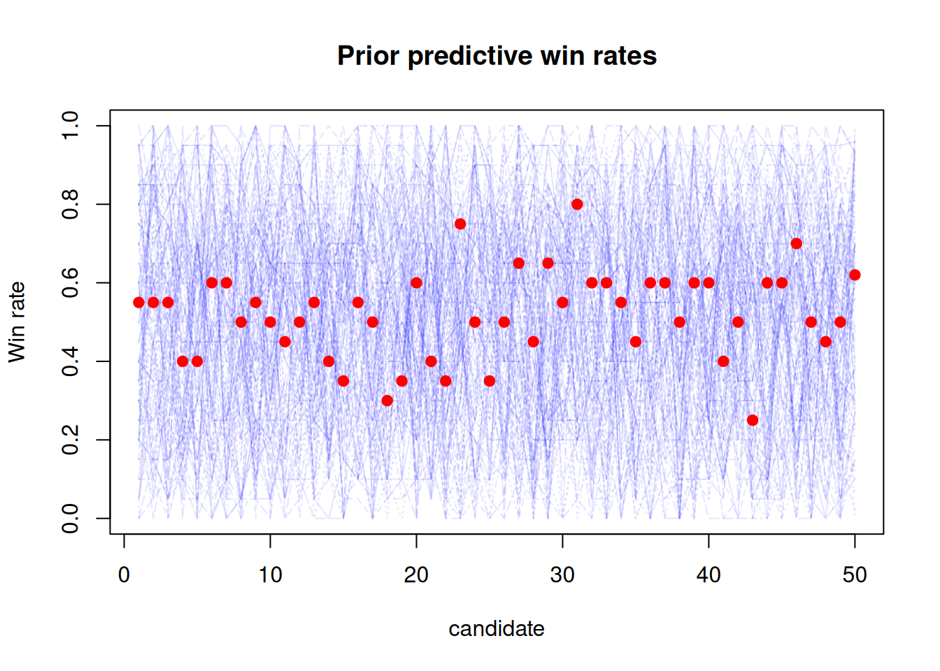
The plot above shows the prior predictive distribution of win rates for the candidates, with the observed win rates overlaid in red. We can see that our priors and model allow for a wide range of observed win rates, so this model seems reasonable.
We are now ready to fit the model using the observed data:
stan_data <- list(
  K = K,
  w = observed_wins,
  l = observed_losses
)

stan_file <- write_stan_file(stan_code)
mod <- cmdstan_model(stan_file)

fit <- mod$sample(
  data = stan_data,
  chains = 4,
  parallel_chains = 4,
  seed = 1405,
  refresh = 0
)
Running MCMC with 4 parallel chains...
Chain 1 finished in 0.6 seconds.
Chain 3 finished in 0.6 seconds.
Chain 4 finished in 0.6 seconds.
Chain 2 finished in 0.7 seconds.
All 4 chains finished successfully.
Mean chain execution time: 0.6 seconds.
Total execution time: 0.8 seconds.We verify that sampling didn’t have any issues:
fit$cmdstan_diagnose()Checking sampler transitions treedepth.
Treedepth satisfactory for all transitions.
Checking sampler transitions for divergences.
No divergent transitions found.
Checking E-BFMI - sampler transitions HMC potential energy.
E-BFMI satisfactory.
Rank-normalized split effective sample size satisfactory for all parameters.
Rank-normalized split R-hat values satisfactory for all parameters.
Processing complete, no problems detected.Posterior summaries
We show the posterior summaries of the winrates for the 10 best candidates based on the median winrate:
posterior_summary <- fit$summary(variables = "winrate_post")

posterior_summary_round <- posterior_summary |>
  mutate(
    across(where(is.numeric), \(x) round(x, 3))
  )

head(
  posterior_summary_round[order(-posterior_summary_round$median), ],
  10
)
# A tibble: 10 × 10
variable mean median sd mad q5 q95 rhat ess_bulk ess_tail
<chr> <dbl> <dbl> <dbl> <dbl> <dbl> <dbl> <dbl> <dbl> <dbl>
1 winrate_post[50] 0.559 0.554 0.038 0.037 0.506 0.628 1.00 2619. 3019
2 winrate_post[31] 0.56 0.55 0.052 0.044 0.495 0.66 1.00 2502. 2547.
3 winrate_post[23] 0.552 0.543 0.048 0.04 0.488 0.643 1 2950. 2197.
4 winrate_post[46] 0.547 0.54 0.046 0.039 0.483 0.631 1 3686. 2990.
5 winrate_post[27] 0.54 0.535 0.045 0.036 0.472 0.62 1.00 3644. 2571.
6 winrate_post[29] 0.54 0.535 0.045 0.037 0.476 0.623 1.00 4150. 2963.
7 winrate_post[7] 0.534 0.532 0.043 0.036 0.468 0.612 1.00 4368. 3115.
8 winrate_post[6] 0.533 0.531 0.044 0.035 0.464 0.61 1.00 4482. 3079.
9 winrate_post[32] 0.533 0.531 0.044 0.035 0.466 0.612 1 4614. 2922.
10 winrate_post[33] 0.533 0.531 0.044 0.034 0.466 0.61 1.00 4334. 2991.The posterior summaries show that candidate 50 has the highest median winrate, closely followed by candidate 31, reflecting the model’s ability to recover the true best candidate.
draws_df <- as_draws_df(
  fit$draws(variables = "winrate_post")
)

p_50_gt_k <- sapply(1:(K - 1), function(k) {
  mean(
    draws_df$`winrate_post[50]` > draws_df[[paste0("winrate_post[", k, "]")]]
  )
})

data.frame(
  candidate = 1:(K - 1),
  P_50_gt_k = p_50_gt_k
) |>
  arrange(P_50_gt_k) |>
  head(10)
candidate P_50_gt_k
1 31 0.50950
2 23 0.56200
3 46 0.60850
4 29 0.64625
5 27 0.64975
6 44 0.67750
7 40 0.68300
8 33 0.68325
9 45 0.68500
10 7 0.68525Recall that candidate \(50\) had a true winrate of \(0.7\), while all other candidates had a true winrate of \(0.5\). The posterior summaries and the probabilities indicate that our hierarchical Bayesian model successfully identifies candidate \(50\) as the best candidate, demonstrating the effectiveness of partial pooling in this context.
Conclusion
Identifying the best candidate, such as a restaurant or a player, based solely on observed outcomes can be misleading, especially when only focusing on the extreme observations. Asking “Is A better than B?” while ignoring all other candidates leads to biased conclusions due to the winner’s curse.
Hierarchical Bayesian multinomial models provide a principled way to address this issue by partially pooling information across candidates. This approach yields more accurate estimates of latent quality and improves the identification of truly top-performing candidates.
Session Info
sessionInfo()R version 4.5.2 (2025-10-31)
Platform: x86_64-pc-linux-gnu
Running under: Linux Mint 22.3
Matrix products: default
BLAS: /usr/lib/x86_64-linux-gnu/openblas-pthread/libblas.so.3
LAPACK: /usr/lib/x86_64-linux-gnu/openblas-pthread/libopenblasp-r0.3.26.so; LAPACK version 3.12.0
locale:
[1] LC_CTYPE=en_US.UTF-8 LC_NUMERIC=C
[3] LC_TIME=en_US.UTF-8 LC_COLLATE=en_US.UTF-8
[5] LC_MONETARY=en_US.UTF-8 LC_MESSAGES=en_US.UTF-8
[7] LC_PAPER=en_US.UTF-8 LC_NAME=C
[9] LC_ADDRESS=C LC_TELEPHONE=C
[11] LC_MEASUREMENT=en_US.UTF-8 LC_IDENTIFICATION=C
time zone: Europe/Copenhagen
tzcode source: system (glibc)
attached base packages:
[1] stats graphics grDevices utils datasets methods base
other attached packages:
[1] cmdstanr_0.9.0 posterior_1.6.1 lubridate_1.9.4 forcats_1.0.1
[5] stringr_1.6.0 dplyr_1.1.4 purrr_1.2.0 readr_2.1.6
[9] tidyr_1.3.2 tibble_3.3.0 ggplot2_4.0.1 tidyverse_2.0.0
loaded via a namespace (and not attached):
[1] tensorA_0.36.2.1 utf8_1.2.6 generics_0.1.4
[4] stringi_1.8.7 hms_1.1.4 digest_0.6.39
[7] magrittr_2.0.4 evaluate_1.0.5 grid_4.5.2
[10] timechange_0.3.0 RColorBrewer_1.1-3 fastmap_1.2.0
[13] jsonlite_2.0.0 processx_3.8.6 backports_1.5.0
[16] ps_1.9.1 scales_1.4.0 codetools_0.2-20
[19] abind_1.4-8 cli_3.6.5 rlang_1.1.6
[22] withr_3.0.2 yaml_2.3.12 otel_0.2.0
[25] tools_4.5.2 tzdb_0.5.0 checkmate_2.3.3
[28] vctrs_0.6.5 R6_2.6.1 matrixStats_1.5.0
[31] lifecycle_1.0.4 htmlwidgets_1.6.4 pkgconfig_2.0.3
[34] pillar_1.11.1 gtable_0.3.6 data.table_1.18.0
[37] glue_1.8.0 xfun_0.55 tidyselect_1.2.1
[40] rstudioapi_0.17.1 knitr_1.51 farver_2.1.2
[43] htmltools_0.5.9 rmarkdown_2.30 compiler_4.5.2
[46] S7_0.2.1 distributional_0.5.0