The Auxiliary Particle Filter differs from the bootstrap filter by incorporating a look-ahead step: particles are reweighted using an approximation of the likelihood of the next observation prior to resampling. This adjustment can help reduce particle degeneracy and, improve filtering efficiency compared to the bootstrap approach.
Arguments
- y
A numeric vector or matrix of observations. Each row represents an observation at a time step. If observations are not equally spaced, use the
obs_timesargument.- num_particles
A positive integer specifying the number of particles.
- init_fn
A function to initialize the particles. Should take `num_particles` and return a matrix or vector of initial states. Additional model parameters can be passed via
....- transition_fn
A function for propagating particles. Should take `particles` and optionally `t`. Additional model parameters via
....- log_likelihood_fn
A function that returns the log-likelihood for each particle given the current observation, particles, and optionally `t`. Additional parameters via
....- aux_log_likelihood_fn
A function that computes the log-likelihood of the next observation given the current particles. It should accept arguments `y`, `particles`, optionally `t`, and any additional model-specific parameters via
.... It returns a numeric vector of log-likelihoods.- obs_times
A numeric vector specifying observation time points. Must match the number of rows in
y, or defaults to1:nrow(y).- resample_algorithm
A character string specifying the filtering resample algorithm:
"SIS"for no resampling,"SISR"for resampling at every time step, or"SISAR"for adaptive resampling when ESS drops belowthreshold. Using"SISR"or"SISAR"to avoid weight degeneracy is recommended. Default is"SISAR".- resample_fn
A string indicating the resampling method:
"stratified","systematic", or"multinomial". Default is"stratified".- threshold
A numeric value specifying the ESS threshold for
"SISAR". Defaults tonum_particles / 2.- return_particles
Logical; if
TRUE, returns the full particle and weight histories.- ...
Additional arguments passed to
init_fn,transition_fn, andlog_likelihood_fn.
Value
A list with components:
- state_est
Estimated states over time (weighted mean of particles).
- ess
Effective sample size at each time step.
- loglike
Total log-likelihood.
- loglike_history
Log-likelihood at each time step.
- algorithm
The filtering algorithm used.
- particles_history
Matrix of particle states over time (if
return_particles = TRUE).- weights_history
Matrix of particle weights over time (if
return_particles = TRUE).
The Auxiliary Particle Filter (APF)
The Auxiliary Particle Filter (APF) was introduced by Pitt and Shephard (1999) to improve upon the standard bootstrap filter by incorporating a look ahead step. Before resampling at time \(t\), particles are weighted by an auxiliary weight proportional to an estimate of the likelihood of the next observation, guiding resampling to favor particles likely to contribute to future predictions.
Specifically, if \(w_{t-1}^i\) are the normalized weights and \(x_{t-1}^i\) are the particles at time \(t-1\), then auxiliary weights are computed as $$ \tilde{w}_t^i \propto w_{t-1}^i \, p(y_t | \mu_t^i), $$ where \(\mu_t^i\) is a predictive summary (e.g., the expected next state) of the particle \(x_{t-1}^i\). Resampling is performed using \(\tilde{w}_t^i\) instead of \(w_{t-1}^i\). This can reduce the variance of the importance weights at time \(t\) and help mitigate particle degeneracy, especially if the auxiliary weights are chosen well.
Default resampling method is stratified resampling, which has lower variance than multinomial resampling (Douc et al., 2005).
Model Specification
Particle filter implementations in this package assume a discrete-time state-space model defined by:
A sequence of latent states \(x_0, x_1, \ldots, x_T\) evolving according to a Markov process.
Observations \(y_1, \ldots, y_T\) that are conditionally independent given the corresponding latent states.
The model is specified as: $$x_0 \sim \mu_\theta$$ $$x_t \sim f_\theta(x_t \mid x_{t-1}), \quad t = 1, \ldots, T$$ $$y_t \sim g_\theta(y_t \mid x_t), \quad t = 1, \ldots, T$$
where \(\theta\) denotes model parameters passed via ....
The user provides the following functions:
init_fn: draws from the initial distribution \(\mu_\theta\).transition_fn: generates or evaluates the transition density \(f_\theta\).weight_fn: evaluates the observation likelihood \(g_\theta\).
References
Pitt, M. K., & Shephard, N. (1999). Filtering via simulation: Auxiliary particle filters. Journal of the American Statistical Association, 94(446), 590–599. doi:10.1080/01621459.1999.10474153
Douc, R., Cappé, O., & Moulines, E. (2005). Comparison of Resampling Schemes for Particle Filtering. Accessible at: https://arxiv.org/abs/cs/0507025
Examples
init_fn <- function(num_particles) rnorm(num_particles, 0, 1)
transition_fn <- function(particles) particles + rnorm(length(particles))
log_likelihood_fn <- function(y, particles) {
dnorm(y, mean = particles, sd = 1, log = TRUE)
}
aux_log_likelihood_fn <- function(y, particles) {
# Predict next state (mean stays same) and compute log p(y | x)
mean_forecast <- particles # since E[x'] = x in this model
dnorm(y, mean = mean_forecast, sd = 1, log = TRUE)
}
y <- cumsum(rnorm(50)) # dummy data
num_particles <- 100
result <- auxiliary_filter(
y = y,
num_particles = num_particles,
init_fn = init_fn,
transition_fn = transition_fn,
log_likelihood_fn = log_likelihood_fn,
aux_log_likelihood_fn = aux_log_likelihood_fn
)
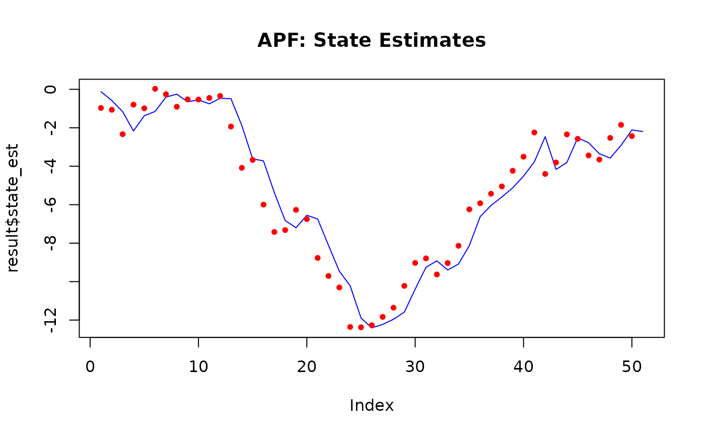
plot(result$state_est,
type = "l", col = "blue", main = "APF: State Estimates",
ylim = range(c(result$state_est, y))
)
points(y, col = "red", pch = 20)
 # ---- With parameters ----
init_fn <- function(num_particles) rnorm(num_particles, 0, 1)
transition_fn <- function(particles, mu) {
particles + rnorm(length(particles), mean = mu)
}
log_likelihood_fn <- function(y, particles, sigma) {
dnorm(y, mean = particles, sd = sigma, log = TRUE)
}
aux_log_likelihood_fn <- function(y, particles, mu, sigma) {
# Forecast mean of x' given x, then evaluate p(y | forecast)
forecast <- particles + mu
dnorm(y, mean = forecast, sd = sigma, log = TRUE)
}
y <- cumsum(rnorm(50)) # dummy data
num_particles <- 100
result <- auxiliary_filter(
y = y,
num_particles = num_particles,
init_fn = init_fn,
transition_fn = transition_fn,
log_likelihood_fn = log_likelihood_fn,
aux_log_likelihood_fn = aux_log_likelihood_fn,
mu = 1,
sigma = 1
)
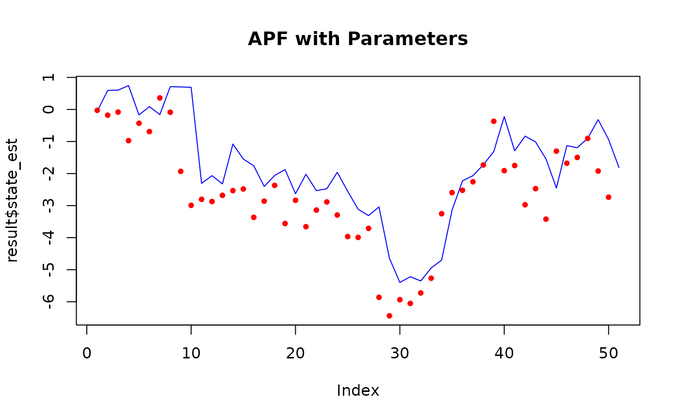
plot(result$state_est,
type = "l", col = "blue", main = "APF with Parameters",
ylim = range(c(result$state_est, y))
)
points(y, col = "red", pch = 20)
# ---- With parameters ----
init_fn <- function(num_particles) rnorm(num_particles, 0, 1)
transition_fn <- function(particles, mu) {
particles + rnorm(length(particles), mean = mu)
}
log_likelihood_fn <- function(y, particles, sigma) {
dnorm(y, mean = particles, sd = sigma, log = TRUE)
}
aux_log_likelihood_fn <- function(y, particles, mu, sigma) {
# Forecast mean of x' given x, then evaluate p(y | forecast)
forecast <- particles + mu
dnorm(y, mean = forecast, sd = sigma, log = TRUE)
}
y <- cumsum(rnorm(50)) # dummy data
num_particles <- 100
result <- auxiliary_filter(
y = y,
num_particles = num_particles,
init_fn = init_fn,
transition_fn = transition_fn,
log_likelihood_fn = log_likelihood_fn,
aux_log_likelihood_fn = aux_log_likelihood_fn,
mu = 1,
sigma = 1
)
plot(result$state_est,
type = "l", col = "blue", main = "APF with Parameters",
ylim = range(c(result$state_est, y))
)
points(y, col = "red", pch = 20)
 # ---- With observation gaps ----
simulate_ssm <- function(num_steps, mu, sigma) {
x <- numeric(num_steps)
y <- numeric(num_steps)
x[1] <- rnorm(1, mean = 0, sd = sigma)
y[1] <- rnorm(1, mean = x[1], sd = sigma)
for (t in 2:num_steps) {
x[t] <- mu * x[t - 1] + sin(x[t - 1]) + rnorm(1, mean = 0, sd = sigma)
y[t] <- x[t] + rnorm(1, mean = 0, sd = sigma)
}
y
}
data <- simulate_ssm(10, mu = 1, sigma = 1)
obs_times <- c(1, 2, 3, 5, 6, 7, 8, 9, 10) # Missing at t = 4
data_obs <- data[obs_times]
init_fn <- function(num_particles) rnorm(num_particles, 0, 1)
transition_fn <- function(particles, mu) {
particles + rnorm(length(particles), mean = mu)
}
log_likelihood_fn <- function(y, particles, sigma) {
dnorm(y, mean = particles, sd = sigma, log = TRUE)
}
aux_log_likelihood_fn <- function(y, particles, mu, sigma) {
forecast <- particles + mu
dnorm(y, mean = forecast, sd = sigma, log = TRUE)
}
num_particles <- 100
result <- auxiliary_filter(
y = data_obs,
num_particles = num_particles,
init_fn = init_fn,
transition_fn = transition_fn,
log_likelihood_fn = log_likelihood_fn,
aux_log_likelihood_fn = aux_log_likelihood_fn,
obs_times = obs_times,
mu = 1,
sigma = 1
)
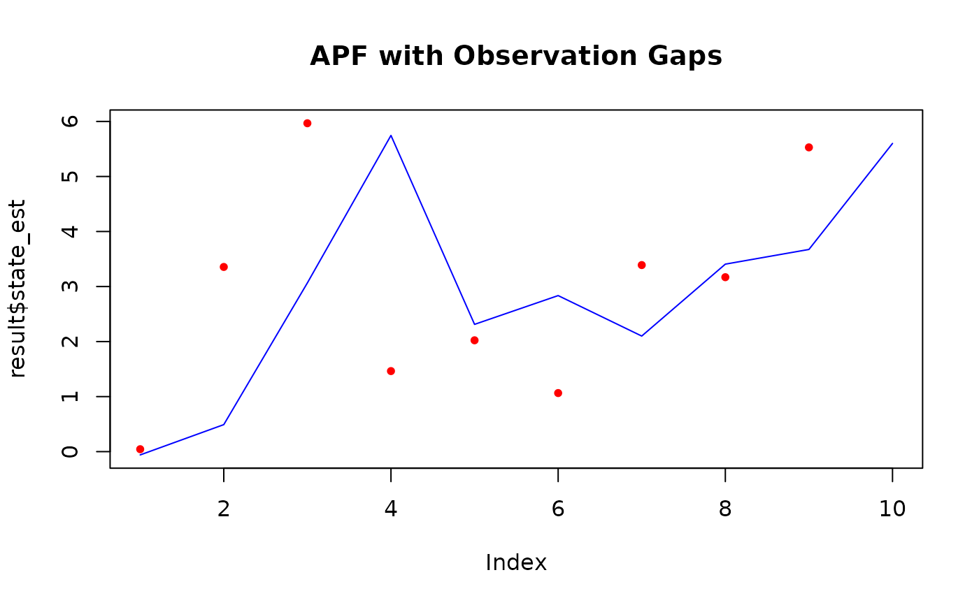
plot(result$state_est,
type = "l", col = "blue", main = "APF with Observation Gaps",
ylim = range(c(result$state_est, data))
)
points(data_obs, col = "red", pch = 20)
# ---- With observation gaps ----
simulate_ssm <- function(num_steps, mu, sigma) {
x <- numeric(num_steps)
y <- numeric(num_steps)
x[1] <- rnorm(1, mean = 0, sd = sigma)
y[1] <- rnorm(1, mean = x[1], sd = sigma)
for (t in 2:num_steps) {
x[t] <- mu * x[t - 1] + sin(x[t - 1]) + rnorm(1, mean = 0, sd = sigma)
y[t] <- x[t] + rnorm(1, mean = 0, sd = sigma)
}
y
}
data <- simulate_ssm(10, mu = 1, sigma = 1)
obs_times <- c(1, 2, 3, 5, 6, 7, 8, 9, 10) # Missing at t = 4
data_obs <- data[obs_times]
init_fn <- function(num_particles) rnorm(num_particles, 0, 1)
transition_fn <- function(particles, mu) {
particles + rnorm(length(particles), mean = mu)
}
log_likelihood_fn <- function(y, particles, sigma) {
dnorm(y, mean = particles, sd = sigma, log = TRUE)
}
aux_log_likelihood_fn <- function(y, particles, mu, sigma) {
forecast <- particles + mu
dnorm(y, mean = forecast, sd = sigma, log = TRUE)
}
num_particles <- 100
result <- auxiliary_filter(
y = data_obs,
num_particles = num_particles,
init_fn = init_fn,
transition_fn = transition_fn,
log_likelihood_fn = log_likelihood_fn,
aux_log_likelihood_fn = aux_log_likelihood_fn,
obs_times = obs_times,
mu = 1,
sigma = 1
)
plot(result$state_est,
type = "l", col = "blue", main = "APF with Observation Gaps",
ylim = range(c(result$state_est, data))
)
points(data_obs, col = "red", pch = 20)