bayesSSM

library(bayesSSM)
library(ggplot2)

We will show how to fit the following SSM model using the bayesSSM package:

$$\begin{align*} X_1 &\sim N(0,\, 1) \\ X_t&=\phi X_{t-1}+\sin(X_{t-1})+\sigma_x V_t, \quad V_t \sim N(0, \, 1) \\ Y_t&=X_t+\sigma_y W_t, \quad W_t \sim N(0, \, 1), \end{align*}$$ that is $X_t$ is a latent state and $Y_t$ is an observed value. The parameters of the model are $\phi$, $\sigma_x$, and $\sigma_y$.

First, we will simulate some data from this model:

set.seed(1405)
t_val <- 50
phi_true <- 0.8
sigma_x_true <- 1
sigma_y_true <- 0.5

x <- numeric(t_val)
y <- numeric(t_val)
x[1] <- rnorm(1)
y[1] <- x[1] + sigma_y_true * rnorm(1)
for (t in 2:t_val) {
  x[t] <- phi_true * x[t - 1] + sin(x[t - 1]) + sigma_x_true * rnorm(1)
  y[t] <- x[t] + sigma_y_true * rnorm(1)
}

Let’s visualize the data:

ggplot() +
  geom_line(aes(x = 1:t_val, y = x), color = "blue", linewidth = 1) + # Latent
  geom_point(aes(x = 1:t_val, y = y), color = "red", size = 2) + # Observed
  labs(
    title = "Simulated Data: Latent State and Observations",
    x = "Time",
    y = "Value",
    caption = "Blue line: Latent state (x), Red points: Observed values (y)"
  ) +
  theme_minimal()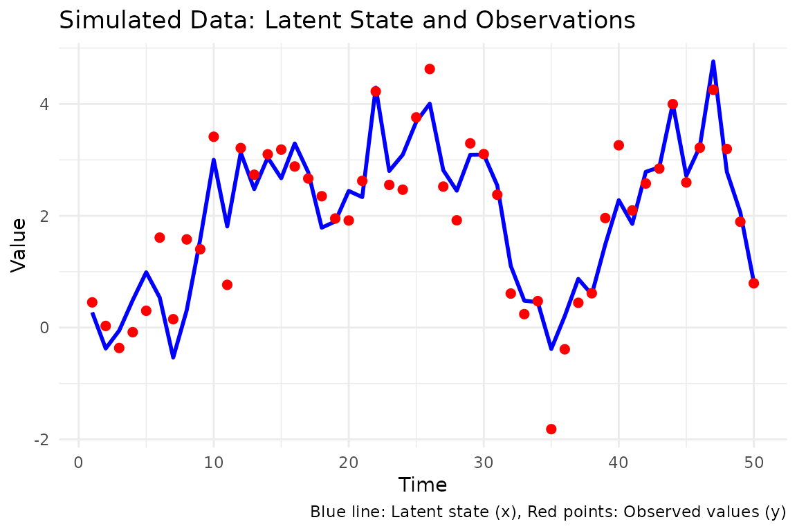

To fit the model using pmmh we need to specify the likelihood initialization, transition, and log-likelihood functions. It’s important that they all take an argument particles, which is a vector of particles, and that the log-likelihood function takes an argument $y$ for the data.

init_fn <- function(particles) {
  rnorm(particles, mean = 0, sd = 1)
}

transition_fn <- function(particles, phi, sigma_x) {
  phi * particles + sin(particles) +
    rnorm(length(particles), mean = 0, sd = sigma_x)
}

log_likelihood_fn <- function(y, particles, sigma_y) {
  dnorm(y, mean = particles, sd = sigma_y, log = TRUE)
}

Since we are interested in Bayesian inference, we need to specify the priors for our parameters. We will use a normal prior for $\phi$ and exponential priors for $\sigma_x$ and $\sigma_y$. pmmh needs the priors to be specified on the $\log$-scale and takes the priors as a list of functions.

log_prior_phi <- function(phi) {
  dunif(phi, min = 0, max = 1, log = TRUE)
}

log_prior_sigma_x <- function(sigma) {
  dexp(sigma, rate = 1, log = TRUE)
}

log_prior_sigma_y <- function(sigma) {
  dexp(sigma, rate = 1, log = TRUE)
}

log_priors <- list(
  phi = log_prior_phi,
  sigma_x = log_prior_sigma_x,
  sigma_y = log_prior_sigma_y
)

The pmmh function automatically tunes the number of particles and proposal distribution for the parameters. The tuning can be modified by the the function default_tune_control.

We fit 2 chains with $m=1000$ iterations for each, with a burn_in of $500$. We also modify the tuning to only use a pilot run of $100$ iterations and $10$ burn-in iterations. In practice you should run more iterations and chains. To improve sampling we specify that proposals for $\sigma_x$ and $\sigma_y$ should be on the $\log$-scale.

result <- pmmh(
  y = y,
  m = 1000,
  init_fn = init_fn,
  transition_fn = transition_fn,
  log_likelihood_fn = log_likelihood_fn,
  log_priors = log_priors,
  pilot_init_params = list(
    c(phi = 0.4, sigma_x = 0.4, sigma_y = 0.4),
    c(phi = 0.8, sigma_x = 0.8, sigma_y = 0.8)
  ),
  burn_in = 500,
  num_chains = 2,
  seed = 1405,
  param_transform = list(
    phi = "identity",
    sigma_x = "log",
    sigma_y = "log"
  ),
  tune_control = default_tune_control(pilot_m = 100, pilot_burn_in = 10),
  verbose = TRUE
)
#> Running chain 1...
#> Running pilot chain for tuning...
#> Pilot chain posterior mean:
#>       phi   sigma_x   sigma_y 
#> 0.8798657 0.9173364 0.5683548
#> Pilot chain posterior covariance (on transformed space):
#>                 phi     sigma_x     sigma_y
#> phi     0.002084208 0.002558793 0.002332220
#> sigma_x 0.002558793 0.008055780 0.006217778
#> sigma_y 0.002332220 0.006217778 0.006318947
#> Using 150 particles for PMMH:
#> Running particle MCMC chain with tuned settings...
#> Running chain 2...
#> Running pilot chain for tuning...
#> Pilot chain posterior mean:
#>       phi   sigma_x   sigma_y 
#> 0.8057224 1.0560141 0.4103715
#> Pilot chain posterior covariance (on transformed space):
#>                 phi     sigma_x     sigma_y
#> phi     0.007080104 0.007619264 0.005622426
#> sigma_x 0.007619264 0.013808487 0.008079961
#> sigma_y 0.005622426 0.008079961 0.006104050
#> Using 160 particles for PMMH:
#> Running particle MCMC chain with tuned settings...
#> PMMH Results Summary:
#>  Parameter Mean   SD Median CI Lower.2.5% CI Upper.97.5% ESS  Rhat
#>        phi 0.82 0.07   0.82          0.66           0.96  30 1.029
#>    sigma_x 0.91 0.11   0.90          0.71           1.18  23 1.075
#>    sigma_y 0.55 0.12   0.54          0.38           0.77   2 1.372
#> Warning in pmmh(y = y, m = 1000, init_fn = init_fn, transition_fn =
#> transition_fn, : Some ESS values are below 400, indicating poor mixing.
#> Consider running the chains for more iterations.
#> Warning in pmmh(y = y, m = 1000, init_fn = init_fn, transition_fn = transition_fn, : 
#> Some Rhat values are above 1.01, indicating that the chains have not converged. 
#> Consider running the chains for more iterations and/or increase burn_in.

We see that the chains gives convergence issues, indicating that we should run it for more iterations, but we ignore this issue in this Vignette.

It automatically prints data frame summarizing the results, which can be printed from any pmmh_output object by calling print.

print(result)
#> PMMH Results Summary:
#>  Parameter Mean   SD Median CI Lower.2.5% CI Upper.97.5% ESS  Rhat
#>        phi 0.82 0.07   0.82          0.66           0.96  30 1.029
#>    sigma_x 0.91 0.11   0.90          0.71           1.18  23 1.075
#>    sigma_y 0.55 0.12   0.54          0.38           0.77   2 1.372

The chains are saved as theta_chain

chains <- result$theta_chain

Let’s collect the chains for phi from the chains and visualize the densities

ggplot(chains, aes(x = phi, fill = factor(chain))) +
  geom_density(alpha = 0.5) +
  labs(
    title = "Density plot of phi chains",
    x = "Value",
    y = "Density",
    fill = "Chain"
  ) +
  theme_minimal()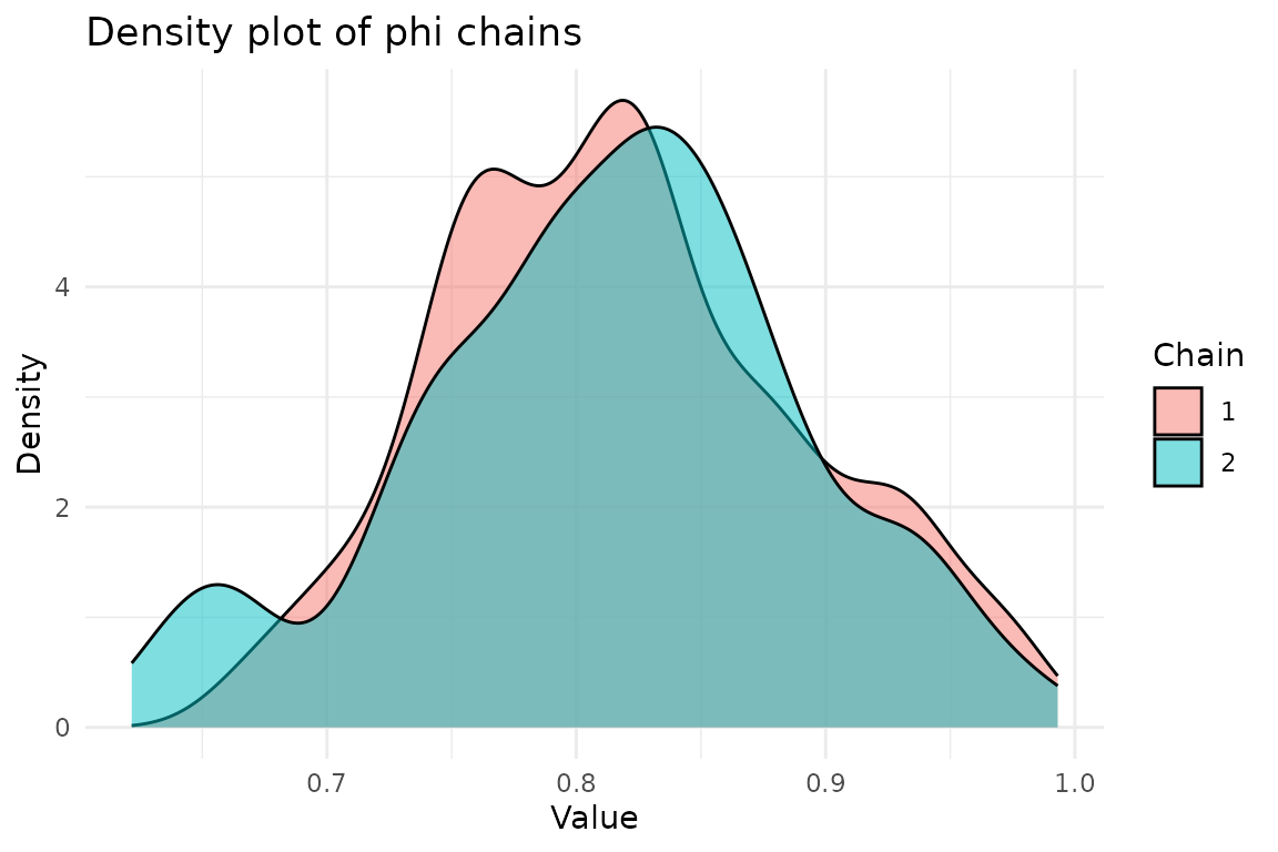

We have now fitted a simple SSM model using bayesSSM. Feel free to explore the package further and try out different models.