Implements a bootstrap particle filter for sequential Bayesian inference in state space models using sequential Monte Carlo methods.
Arguments
- y
A numeric vector or matrix of observations. Each row represents an observation at a time step. If observations are not equally spaced, use the
obs_timesargument.- num_particles
A positive integer specifying the number of particles.
- init_fn
A function to initialize the particles. Should take `num_particles` and return a matrix or vector of initial states. Additional model parameters can be passed via
....- transition_fn
A function for propagating particles. Should take `particles` and optionally `t`. Additional model parameters via
....- log_likelihood_fn
A function that returns the log-likelihood for each particle given the current observation, particles, and optionally `t`. Additional parameters via
....- obs_times
A numeric vector specifying observation time points. Must match the number of rows in
y, or defaults to1:nrow(y).- resample_algorithm
A character string specifying the filtering resample algorithm:
"SIS"for no resampling,"SISR"for resampling at every time step, or"SISAR"for adaptive resampling when ESS drops belowthreshold. Using"SISR"or"SISAR"to avoid weight degeneracy is recommended. Default is"SISAR".- resample_fn
A string indicating the resampling method:
"stratified","systematic", or"multinomial". Default is"stratified".- threshold
A numeric value specifying the ESS threshold for
"SISAR". Defaults tonum_particles / 2.- return_particles
Logical; if
TRUE, returns the full particle and weight histories.- ...
Additional arguments passed to
init_fn,transition_fn, andlog_likelihood_fn.
Value
A list with components:
- state_est
Estimated states over time (weighted mean of particles).
- ess
Effective sample size at each time step.
- loglike
Total log-likelihood.
- loglike_history
Log-likelihood at each time step.
- algorithm
The filtering algorithm used.
- particles_history
Matrix of particle states over time (if
return_particles = TRUE).- weights_history
Matrix of particle weights over time (if
return_particles = TRUE).
The Effective Sample Size (ESS) is defined as
$$ESS = \left(\sum_{i=1}^{n} w_i^2\right)^{-1},$$ where \(w_i\) are the normalized weights of the particles.
Default resampling method is stratified resampling, which has lower variance than multinomial resampling (Douc et al., 2005).
Model Specification
Particle filter implementations in this package assume a discrete-time state-space model defined by:
A sequence of latent states \(x_0, x_1, \ldots, x_T\) evolving according to a Markov process.
Observations \(y_1, \ldots, y_T\) that are conditionally independent given the corresponding latent states.
The model is specified as: $$x_0 \sim \mu_\theta$$ $$x_t \sim f_\theta(x_t \mid x_{t-1}), \quad t = 1, \ldots, T$$ $$y_t \sim g_\theta(y_t \mid x_t), \quad t = 1, \ldots, T$$
where \(\theta\) denotes model parameters passed via ....
The user provides the following functions:
init_fn: draws from the initial distribution \(\mu_\theta\).transition_fn: generates or evaluates the transition density \(f_\theta\).weight_fn: evaluates the observation likelihood \(g_\theta\).
References
Gordon, N. J., Salmond, D. J., & Smith, A. F. M. (1993). Novel approach to nonlinear/non-Gaussian Bayesian state estimation. IEE Proceedings F (Radar and Signal Processing), 140(2), 107–113. doi:10.1049/ip-f-2.1993.0015
Douc, R., Cappé, O., & Moulines, E. (2005). Comparison of Resampling Schemes for Particle Filtering. Accessible at: https://arxiv.org/abs/cs/0507025
Examples
init_fn <- function(num_particles) rnorm(num_particles, 0, 1)
transition_fn <- function(particles) particles + rnorm(length(particles))
log_likelihood_fn <- function(y, particles) {
dnorm(y, mean = particles, sd = 1, log = TRUE)
}
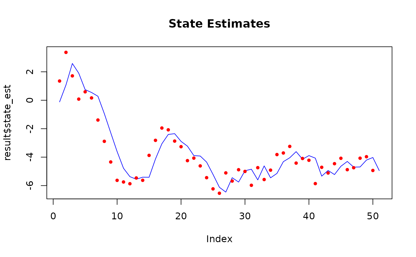
y <- cumsum(rnorm(50)) # dummy data
num_particles <- 100
# Run the particle filter using default settings.
result <- bootstrap_filter(
y = y,
num_particles = num_particles,
init_fn = init_fn,
transition_fn = transition_fn,
log_likelihood_fn = log_likelihood_fn
)
plot(result$state_est,
type = "l", col = "blue", main = "State Estimates",
ylim = range(c(result$state_est, y))
)
points(y, col = "red", pch = 20)
 # With parameters
init_fn <- function(num_particles) rnorm(num_particles, 0, 1)
transition_fn <- function(particles, mu) {
particles + rnorm(length(particles), mean = mu)
}
log_likelihood_fn <- function(y, particles, sigma) {
dnorm(y, mean = particles, sd = sigma, log = TRUE)
}
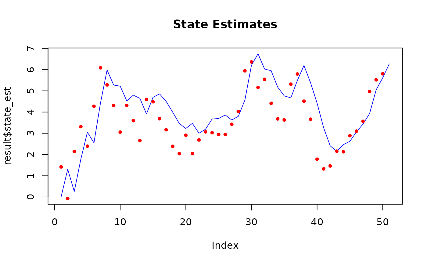
y <- cumsum(rnorm(50)) # dummy data
num_particles <- 100
# Run the bootstrap particle filter using default settings.
result <- bootstrap_filter(
y = y,
num_particles = num_particles,
init_fn = init_fn,
transition_fn = transition_fn,
log_likelihood_fn = log_likelihood_fn,
mu = 1,
sigma = 1
)
plot(result$state_est,
type = "l", col = "blue", main = "State Estimates",
ylim = range(c(result$state_est, y))
)
points(y, col = "red", pch = 20)
# With parameters
init_fn <- function(num_particles) rnorm(num_particles, 0, 1)
transition_fn <- function(particles, mu) {
particles + rnorm(length(particles), mean = mu)
}
log_likelihood_fn <- function(y, particles, sigma) {
dnorm(y, mean = particles, sd = sigma, log = TRUE)
}
y <- cumsum(rnorm(50)) # dummy data
num_particles <- 100
# Run the bootstrap particle filter using default settings.
result <- bootstrap_filter(
y = y,
num_particles = num_particles,
init_fn = init_fn,
transition_fn = transition_fn,
log_likelihood_fn = log_likelihood_fn,
mu = 1,
sigma = 1
)
plot(result$state_est,
type = "l", col = "blue", main = "State Estimates",
ylim = range(c(result$state_est, y))
)
points(y, col = "red", pch = 20)
 # With observations gaps
init_fn <- function(num_particles) rnorm(num_particles, 0, 1)
transition_fn <- function(particles, mu) {
particles + rnorm(length(particles), mean = mu)
}
log_likelihood_fn <- function(y, particles, sigma) {
dnorm(y, mean = particles, sd = sigma, log = TRUE)
}
# Generate data using DGP
simulate_ssm <- function(num_steps, mu, sigma) {
x <- numeric(num_steps)
y <- numeric(num_steps)
x[1] <- rnorm(1, mean = 0, sd = sigma)
y[1] <- rnorm(1, mean = x[1], sd = sigma)
for (t in 2:num_steps) {
x[t] <- mu * x[t - 1] + sin(x[t - 1]) + rnorm(1, mean = 0, sd = sigma)
y[t] <- x[t] + rnorm(1, mean = 0, sd = sigma)
}
y
}
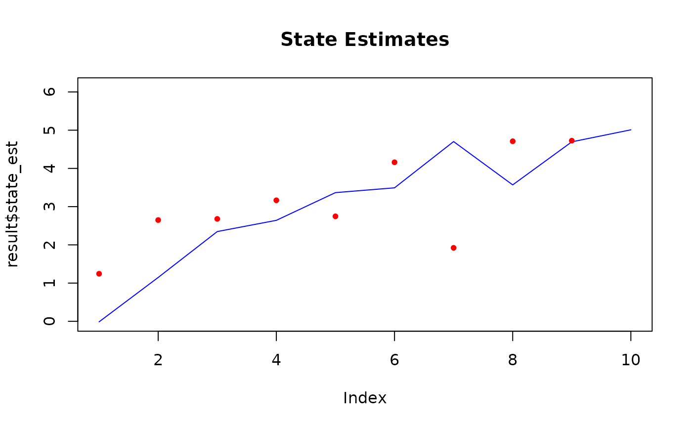
data <- simulate_ssm(10, mu = 1, sigma = 1)
# Suppose we have data for t=1,2,3,5,6,7,8,9,10 (i.e., missing at t=4)
obs_times <- c(1, 2, 3, 5, 6, 7, 8, 9, 10)
data_obs <- data[obs_times]
num_particles <- 100
# Specify observation times in the bootstrap particle filter using obs_times
result <- bootstrap_filter(
y = data_obs,
num_particles = num_particles,
init_fn = init_fn,
transition_fn = transition_fn,
log_likelihood_fn = log_likelihood_fn,
obs_times = obs_times,
mu = 1,
sigma = 1,
)
plot(result$state_est,
type = "l", col = "blue", main = "State Estimates",
ylim = range(c(result$state_est, data))
)
points(data_obs, col = "red", pch = 20)
# With observations gaps
init_fn <- function(num_particles) rnorm(num_particles, 0, 1)
transition_fn <- function(particles, mu) {
particles + rnorm(length(particles), mean = mu)
}
log_likelihood_fn <- function(y, particles, sigma) {
dnorm(y, mean = particles, sd = sigma, log = TRUE)
}
# Generate data using DGP
simulate_ssm <- function(num_steps, mu, sigma) {
x <- numeric(num_steps)
y <- numeric(num_steps)
x[1] <- rnorm(1, mean = 0, sd = sigma)
y[1] <- rnorm(1, mean = x[1], sd = sigma)
for (t in 2:num_steps) {
x[t] <- mu * x[t - 1] + sin(x[t - 1]) + rnorm(1, mean = 0, sd = sigma)
y[t] <- x[t] + rnorm(1, mean = 0, sd = sigma)
}
y
}
data <- simulate_ssm(10, mu = 1, sigma = 1)
# Suppose we have data for t=1,2,3,5,6,7,8,9,10 (i.e., missing at t=4)
obs_times <- c(1, 2, 3, 5, 6, 7, 8, 9, 10)
data_obs <- data[obs_times]
num_particles <- 100
# Specify observation times in the bootstrap particle filter using obs_times
result <- bootstrap_filter(
y = data_obs,
num_particles = num_particles,
init_fn = init_fn,
transition_fn = transition_fn,
log_likelihood_fn = log_likelihood_fn,
obs_times = obs_times,
mu = 1,
sigma = 1,
)
plot(result$state_est,
type = "l", col = "blue", main = "State Estimates",
ylim = range(c(result$state_est, data))
)
points(data_obs, col = "red", pch = 20)