sir-model

library(bayesSSM)
library(ggplot2)
library(tidyr)
library(extraDistr)
set.seed(1405)

SIR model

We will implement the following SIR model. Consider a closed population of size $N$ (i.e. no births, deaths or migration) and three compartments: susceptible, infected and recovered. We assume that initially every individual is susceptible except for $m$ infected individuals.

We assume the any indivudlas infectious period, contacts with any given member of the population occur according to a time-homogeneous Poisson process with rate $\lambda/n$, where $\lambda > 0$ and $n$ the number of susceptible. When a susceptible individual is contacted, they become infected instantaneously and subsequently follow the same infectious process.

We let the distribution of the infection period, $I$ be exponential distributed: $$I \sim \text{Exp}(\gamma)$$ where $\gamma > 0$.

Let $S(t)$ denote the number of susceptible individuals and $I(t)$ denote the number of infectious individuals at time $t \geq 0$. Note, that under these assumptions $$\{(S(t), I(t)) : t \geq 0\}$$ is a Markov process, since the infection event is exponential distributed (since time to next event of a Poisson process is exponential) and so is the removal event, thus memoryless.

The infection and removal events have the following rates:

• Infection Event: The transition $$(s,i) \to (s-1, i+1)$$ occurs at rate $$\frac{\lambda}{n}\, s\, i,$$ for $s > 0$ and $i > 0$.

• Removal Event: The transition $$(s,i) \to (s, i-1)$$ occurs at rate $$\gamma\, i,$$ for $i > 0$.

Partial observations and noisy measurements

Suppose we only observe the initial state and the number of infectious individuals, $I(t)$, at discrete times $t = 0, 1, \ldots, T$. We assume that the true number of infectious individuals is a latent state and we observe a noisy version of this state, that could either be higher or lower (often it is lower). We model this as a Poisson distribution: $$Y_t \mid I(t) \sim \operatorname{Pois}(I(t)),$$ where $\phi > 0$ is the overdispersion parameter.

Simulate data

We will simulate data from the SIR model with the following parameters: - At $t=0$ we have $S(0) = 90$, $I(0) = 10$ and $R(0) = 0$. - Infection rate $\lambda=1.5$ and removal rate $\gamma=0.5$. - $\phi=3$ for the overdispersion parameter. - We observe the number of infectious individuals at times $t=0, 1, \ldots, 10$. representing observations for each day.

We can simulate using the fact that we have two independent exponential distribution, so an event occurs at rate of the sum of the rates.

# --- Simulation settings and true parameters ---
n_total <- 500 # Total population size
init_infected <- 70 # Initially infectious individuals
init_state <- c(n_total - init_infected, init_infected) # (s, i) at time 0
t_max <- 10 # Total number of days to simulate
true_lambda <- 0.5 # True infection parameter
true_gamma <- 0.2 # True removal parameter
phi_true <- 1 # True dispersion parameter for negative binomial
p_true <- 0.9 # True probability for binomial

# --- Functions for simulating the epidemic ---

# Gillespie simulation: simulate from current state for a time interval
gillespie_step <- function(state, t_end, lambda, gamma, n_total) {
  t <- 0
  s <- state[1]
  i <- state[2]
  while (t < t_end && i > 0) {
    rate_infection <- (lambda / n_total) * s * i
    rate_removal <- gamma * i
    rate_total <- rate_infection + rate_removal
    if (rate_total <= 0) break
    dt <- rexp(1, rate_total)
    if (t + dt > t_end) break
    t <- t + dt
    # Decide which event occurs:
    if (runif(1) < rate_infection / rate_total) {
      # Infection event (only possible if s > 0)
      if (s > 0) {
        s <- s - 1
        i <- i + 1
      }
    } else {
      # Removal event
      i <- i - 1
    }
  }
  c(s, i)
}

# Simulate epidemic trajectory using Gillespie
simulate_epidemic_gillespie <- function(
    n_total, init_infected, lambda, gamma, t_max) {
  states <- matrix(0, nrow = t_max + 1, ncol = 2)
  # initial state at t = 0
  states[1, ] <- c(n_total - init_infected, init_infected)
  state <- states[1, ]
  for (t in 1:t_max) {
    state <- gillespie_step(state, 1, lambda, gamma, n_total)
    states[t + 1, ] <- state
  }
  states
}

Now, we generate some data:

# Simulate a "true" epidemic dataset
true_states <- simulate_epidemic_gillespie(
  n_total, init_infected, true_lambda, true_gamma, t_max
)
latent_i <- true_states[, 2]

# Poisson
observations <- rpois(length(latent_i), lambda = latent_i)

# Display simulated data: time, susceptible, latent infectious, observed counts
print(data.frame(
  time = 0:t_max, s = true_states[, 1], i = true_states[, 2], y = observations
))
#>    time   s   i   y
#> 1     0 430  70  83
#> 2     1 391  88  82
#> 3     2 348 113  97
#> 4     3 307 132 122
#> 5     4 266 147 138
#> 6     5 221 164 161
#> 7     6 183 171 166
#> 8     7 155 159 152
#> 9     8 137 143 151
#> 10    9 118 139 141
#> 11   10 107 121 122

And plot it:

# Function to create a tidy dataset for ggplot
prepare_data_for_plot <- function(states, observations, t_max) {
  # Organize the data into a tidy format
  data <- data.frame(
    time = 0:t_max,
    s = states[, 1],
    i = states[, 2],
    y = observations
  )

  # Convert to long format for ggplot
  data_long <- data %>%
    gather(key = "state", value = "count", -time)

  data_long
}

# Function to plot the epidemic data
plot_epidemic_data <- function(data_long, t_max) {
  ggplot(data_long, aes(x = time, y = count, color = state)) +
    geom_line(linewidth = 1.2) +
    scale_color_manual(values = c("s" = "blue", "i" = "red", "y" = "green")) +
    labs(
      x = "Time (Days)", y = "Count",
      title = "Susceptible, Infected, and Observed Counts"
    ) +
    theme_minimal() +
    theme(legend.title = element_blank()) +
    scale_x_continuous(breaks = 0:t_max) +
    theme(
      axis.title = element_text(size = 12),
      plot.title = element_text(size = 14, hjust = 0.5)
    )
}

# Prepare data for plotting
data_long <- prepare_data_for_plot(true_states, observations, t_max)

# Plot the results
plot_epidemic_data(data_long, t_max)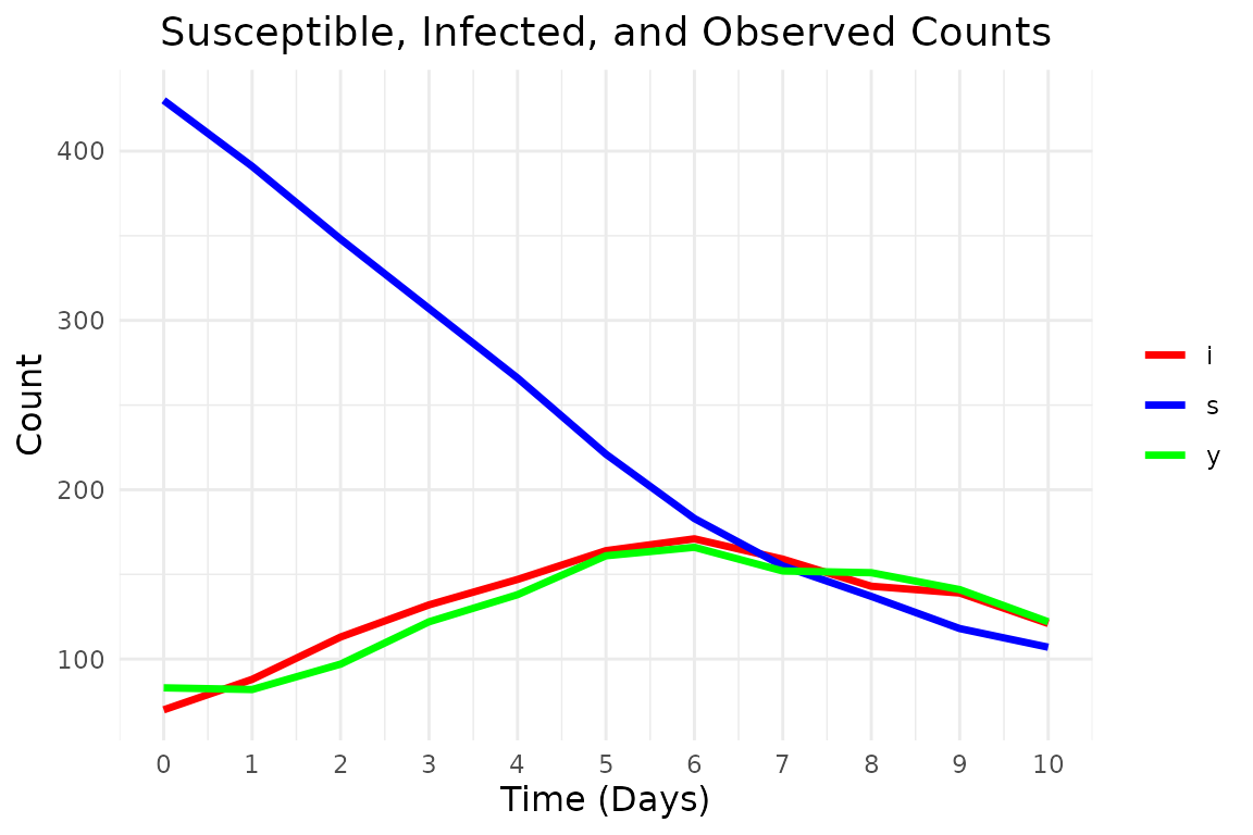

We are interested in performing Bayesian inference in this setup. So we define our priors as We define the priors for $\lambda, \gamma$ and $\phi$ as $$\begin{align*} \lambda \sim \text{half-}N(1), \\ \gamma \sim \text{half-}N(2), \\ \frac{1}{\sqrt{\phi}} \sim \text{half-}N(1), \end{align*}$$ where $\text{half-}N(a)$ denotes a half-normal distribution with mean $0$ and standard deviation $a$. The prior for the over-dispersion parameter $\phi$ follows the recommendation by https://mc-stan.org/users/documentation/case-studies.

We define these priors, where since we specify the prior for $\phi$ on another scale we need to include the Jacobian term in the likelihood.

# Define the log-prior for the parameters
log_prior_lambda <- function(lambda) {
  extraDistr::dhnorm(lambda, sigma = 1, log = TRUE)
}

log_prior_gamma <- function(gamma) {
  extraDistr::dhnorm(gamma, sigma = 2, log = TRUE)
}

log_prior_phi <- function(phi) {
  if (phi <= 0) {
    return(-Inf)
  } # Ensure phi is positive

  # Jacobian: |d(1/sqrt(phi))/dphi| = 1/(2 * phi^(3/2))
  log_jacobian <- -log(2) - 1.5 * log(phi)
  extraDistr::dhnorm(1 / sqrt(phi), sigma = 1, log = TRUE) + log_jacobian
}

log_prior_p <- function(p) {
  dunif(p, 0, 1, log = TRUE)
}

log_priors <- list(
  lambda = log_prior_lambda,
  gamma = log_prior_gamma
)

We now define the initial state, transition and likelihood functions for the SIR model.

init_fn_epidemic <- function(particles) {
  # Return a matrix with particles rows; each row is the initial state (s, i)
  matrix(rep(init_state, each = particles), nrow = particles, byrow = FALSE)
}

transition_fn_gillespie <- function(particles, lambda, gamma) {
  new_particles <- t(apply(particles, 1, function(state) {
    s <- state[1]
    i <- state[2]
    if (i == 0) {
      return(c(s, i))
    }
    gillespie_step(state, t_end = 1, lambda, gamma, n_total)
  }))
  new_particles
}

log_likelihood_fn_epidemic <- function(y, particles) {
  # particles is expected to be a matrix with columns (s, i)
  dpois(y, lambda = particles[, 2], log = TRUE)
}

Now we can run the PMMH algorithm to estimate the parameters. For this vignette we only use a small number of iterations (1000) and 2 chains (and we also modify the tuning to only use 100 iterations with a burn-in of 10). In practice, these should be much higher.

result <- bayesSSM::pmmh(
  y = observations,
  m = 1000,
  init_fn = init_fn_epidemic,
  transition_fn = transition_fn_gillespie,
  log_likelihood_fn = log_likelihood_fn_epidemic,
  log_priors = log_priors,
  pilot_init_params = list(
    c(lambda = 0.5, gamma = 0.5),
    c(lambda = 1, gamma = 1)
  ),
  burn_in = 200,
  num_chains = 2,
  param_transform = list(lambda = "log", gamma = "log"),
  tune_control = default_tune_control(pilot_m = 100, pilot_burn_in = 10),
  verbose = TRUE,
  seed = 1405,
)
#> Running chain 1...
#> Running pilot chain for tuning...
#> Pilot chain posterior mean:
#>    lambda     gamma 
#> 0.5321679 0.2066975
#> Pilot chain posterior covariance (on transformed space):
#>              lambda        gamma
#> lambda 0.0044377970 0.0006943389
#> gamma  0.0006943389 0.0001268842
#> Using 50 particles for PMMH:
#> Running particle MCMC chain with tuned settings...
#> Running chain 2...
#> Running pilot chain for tuning...
#> Pilot chain posterior mean:
#>    lambda     gamma 
#> 0.5481187 0.2116892
#> Pilot chain posterior covariance (on transformed space):
#>               lambda         gamma
#> lambda  6.046094e-05 -7.679654e-05
#> gamma  -7.679654e-05  9.754576e-05
#> Using 50 particles for PMMH:
#> Running particle MCMC chain with tuned settings...
#> PMMH Results Summary:
#>  Parameter Mean   SD Median CI Lower.2.5% CI Upper.97.5% ESS  Rhat
#>     lambda 0.55 0.06   0.55          0.42           0.69 156 1.019
#>      gamma 0.21 0.02   0.21          0.18           0.25  62 1.033
#> Warning in bayesSSM::pmmh(y = observations, m = 1000, init_fn =
#> init_fn_epidemic, : Some ESS values are below 400, indicating poor mixing.
#> Consider running the chains for more iterations.
#> Warning in bayesSSM::pmmh(y = observations, m = 1000, init_fn = init_fn_epidemic, : 
#> Some Rhat values are above 1.01, indicating that the chains have not converged. 
#> Consider running the chains for more iterations and/or increase burn_in.

We get convergence warnings as expected, but we still recover the true values.

We can access the chains and plot the densities:

chains <- result$theta_chain

For $\lambda$:

ggplot(chains, aes(x = lambda, fill = factor(chain))) +
  geom_density(alpha = 0.5) +
  labs(
    title = "Density plot of lambda chains",
    x = "Value",
    y = "Density",
    fill = "Chain"
  ) +
  theme_minimal()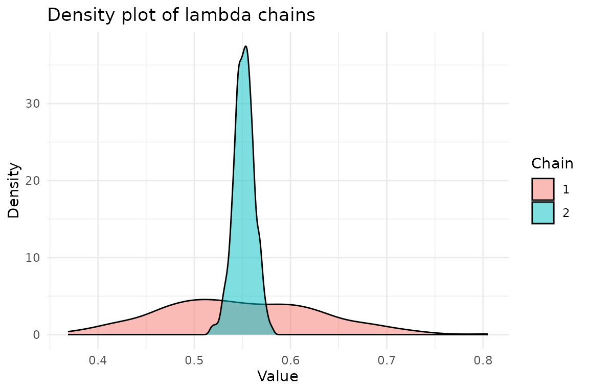

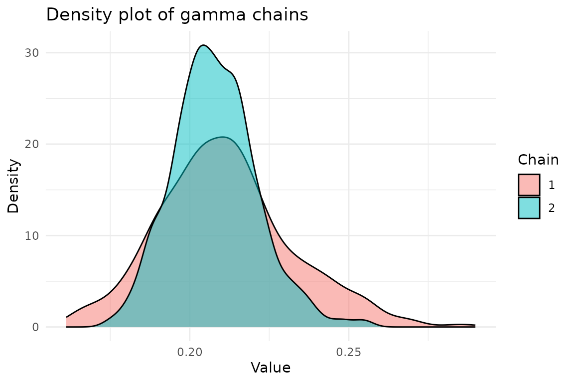
And for $\gamma$:

ggplot(chains, aes(x = gamma, fill = factor(chain))) +
  geom_density(alpha = 0.5) +
  labs(
    title = "Density plot of gamma chains",
    x = "Value",
    y = "Density",
    fill = "Chain"
  ) +
  theme_minimal()